Lecture 7: Visualization and Reporting with R

By now you should be familiar with most of the core functionality of the R programming language. We can perform simulations, graph results, create summary statistics, export our results to files and accomplish almost any programming feat by simply using the base installation of R. In this lecture I want to introduce a few tools (libraries) that extend R’s reach. Especially, in terms of producing robust and elegant visualizations and drafting reproducible reports.

Graphing

All of our graphing needs up to this point have been met by the plot(), lines() and abline() functions. We can do better than this.

Hadley Wickham has created a great library that takes graphing/plotting in R to a whole new level. The library is called ggplot2 and much more information about it can be found here: ggplot2 examples.

According to the ggplot2 website: “ggplot2 is a plotting system for R, based on the grammar of graphics, which tries to take the good parts of base and lattice graphics and none of the bad parts. It takes care of many of the fiddly details that make plotting a hassle (like drawing legends) as well as providing a powerful model of graphics that makes it easy to produce complex multi-layered graphics.”

Let’s take a look at a few examples. (I will closely follow the examples presented here.)

qplot()

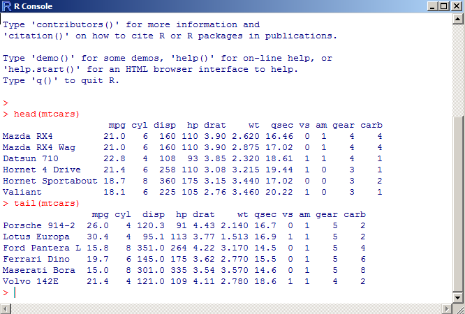
We will be utilizing the mtcars data frame that is already accessible through R. Here’s what it looks like:

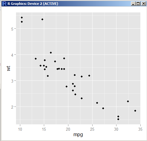
The qplot() function is similar to the plot() function in many respects.

 require(ggplot2)
 qplot(mpg, wt, data = mtcars)

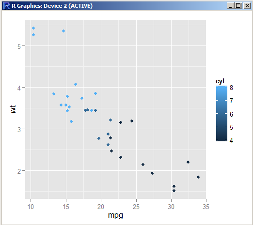
 # Add different colors based on the cylinder type 
 qplot(mpg, wt, data = mtcars, colour = cyl)

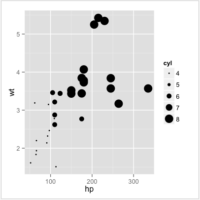
 # Different styling based on the cylinder type
 qplot(mpg, wt, data = mtcars, size = cyl)

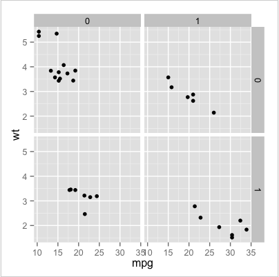
 # One or two sided faceting formula
 qplot(mpg, wt, data = mtcars, facets = vs ~ am)

Graphics grammar syntax

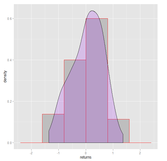
Let’s take a look at a more interesting example that leverages the graphics grammar paradigm. More information on what a graphics grammar is can be found here.

 stocks <- data.frame(signal = sample(c("Buy", "Sell"), 100, replace = TRUE), returns = rnorm(100, 0, 0.6))
 
obj <- ggplot(stocks, aes(x=returns))
obj <- obj + geom_histogram(aes(y=..density..), binwidth=.8, colour="red", fill="grey") 
obj <- obj + geom_density(alpha=.2, fill="purple")
obj

Reporting

No matter how sophisticated or elegant your statistical analysis happens to be, if you can’t report your results in a meaningful and reproducible way to your management or end-users of your research, your conclusions will be lost. The following steps outline one easy way for weaving together your analytics with your reporting and presenting the end result in a clean and comprehensive manner.

Rstudio

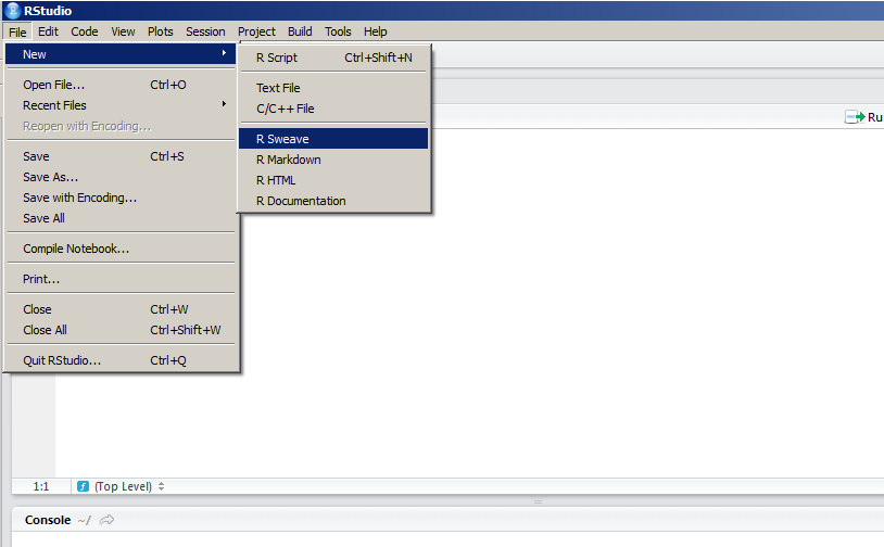
Rstudio is currently one of the best IDE’s (Integrated Development Environment) available for the R language. It is 100% free, is cross-platform (meaning that it works on windows, linux and mac machines) and enables R programmers to become more productive by providing them with all the functionality they could possibly need within the IDE.

Rstudio can be downloaded from Rstudio.com. Rstudio bundles various third party libraries that we will be utilizing in this lecture. One of them is knitr. This library was created by Yihui Xie and allows one to create PDF reports that include embedded R code along with LaTeX formatting. To find more about what LaTeX is and how it can help you write better documents, click here: LaTeX details.

In order to use the knitr library, LaTeX needs to be installed on your computer. If you are using a windows machine, you can obtain LaTeX from here: LaTeX for Windows. If you are using a mac, you can get LaTeX from here: LaTeX for Mac. Once you have downloaded and installed Rstudio, there is no need to install knitr. It is already part of the Rstudio installation.

How to create a simple .pdf report with Rstudio

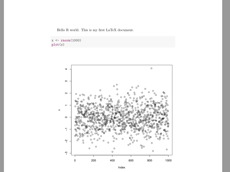
Let’s take this a step further and add some R code and some formatting into the mix. Here’s what the complete document contents should look like:

 \documentclass{article}
 
 \begin{document}
 
   Hello R world. This is my first LaTeX document. 
 
   <<echo = TRUE, message = FALSE>>=
 
    x <- rnorm(1000)
    plot(x)
 
   @
 
 \end{document}

The echo = TRUE command tells knitr to output the code to the pdf file. Not only is the code echoed to the user, it is also executed and the result prints to the pdf document.

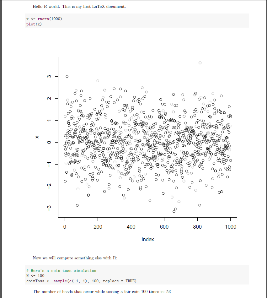
Here’s a slightly more complicated example that passes a variable calculated from R back to the LaTeX text. I have also added some formatting to the pdf document itself for adjusting the margins slightly. Notice the use of the Sexpr command in the example below:

 \documentclass{article}
 
  \usepackage[
   top    = 1.00cm,
   bottom = 1.00cm,
   left   = 2.00cm,
   right  = 1.50cm]{geometry}
 
 \begin{document}
 
   Hello R world. This is my first LaTeX document. 
 
   <<echo = TRUE, message = FALSE>>=
 
    x <- rnorm(1000)
    plot(x)
   @
 
   Now we will compute something else with R:
 
   <<echo = TRUE, message = FALSE>>=
 
   # Here's a coin toss simulation
   N        <- 100
   coinToss <- sample(c(-1, 1), 100, replace = TRUE)
 
   @
 
  The number of heads that occur while tossing 
  a fair coin \Sexpr{N} times is: \Sexpr{length(which(coinToss == 1))}
 
 \end{document}

Formatting a LaTeX document is something that we have not covered in this class. Here’s a cheat sheet that might come in handy when working with LaTeX syntax.

Lecture 7 – Visualization and Reporting with R